[1] "hello world"tidyverse for data analysis
remixed from Claus O. Wilke’s SDS375 course and Andrew P. Bray’s quarto workshop
Let’s take a poll
Go to the event on wooclap

Positron
Let’s take a poll
Go to the event on wooclap
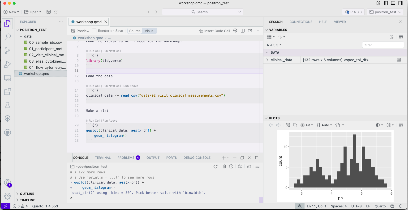
Quarto’s Code Chunk
You can quickly insert chunks like these into your file with
- the keyboard shortcut Ctrl + Alt + I (OS X: Shift + Command + I)
- the Add Chunk
![]() command in the editor toolbar
command in the editor toolbar
- or by typing the chunk delimiters
```{r}```
Example chunk:
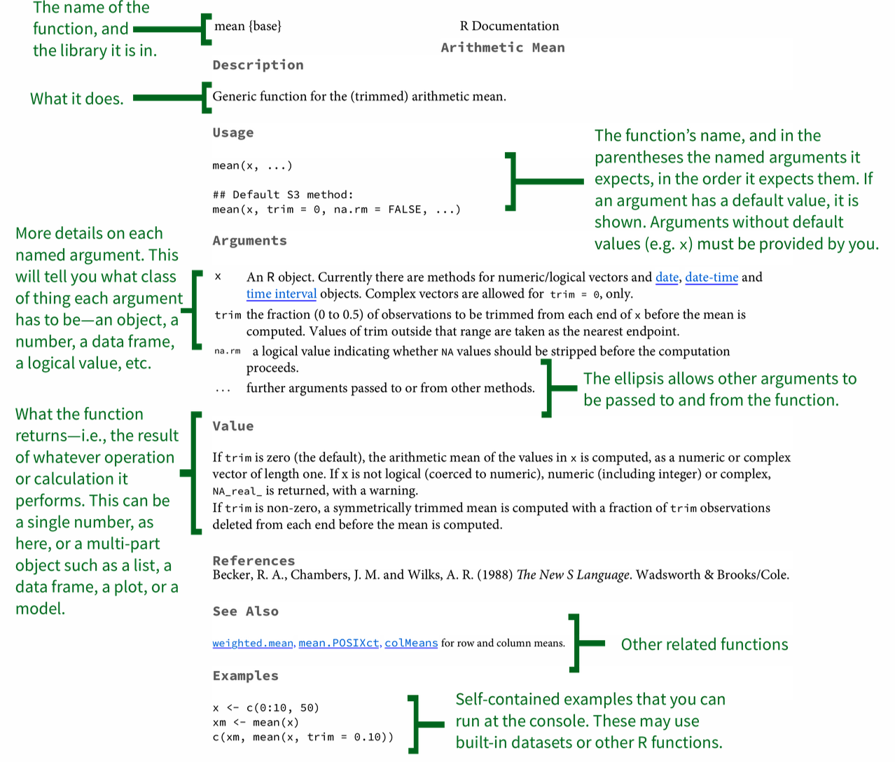
Getting help with functions
Type ?str_c in the console to get a help page. check out this guide on how to read the R help pages.
Google! Add “tidyverse” to search queries to get more relevant results.
phind.com and chat.deepseek.com are good free AI services for getting help with code.
The pipe %>% feeds data into functions

The pipe %>% feeds data into functions

Since R 4.1: Native pipe |>
Pick rows from a table: filter()

Pick columns from a table: select()

Sort the rows in a table: arrange()

Let’s take a poll
Go to the event on wooclap
M2. Does filter get rid of rows that match TRUE, or keep rows that match TRUE?
Make a new table column: mutate()

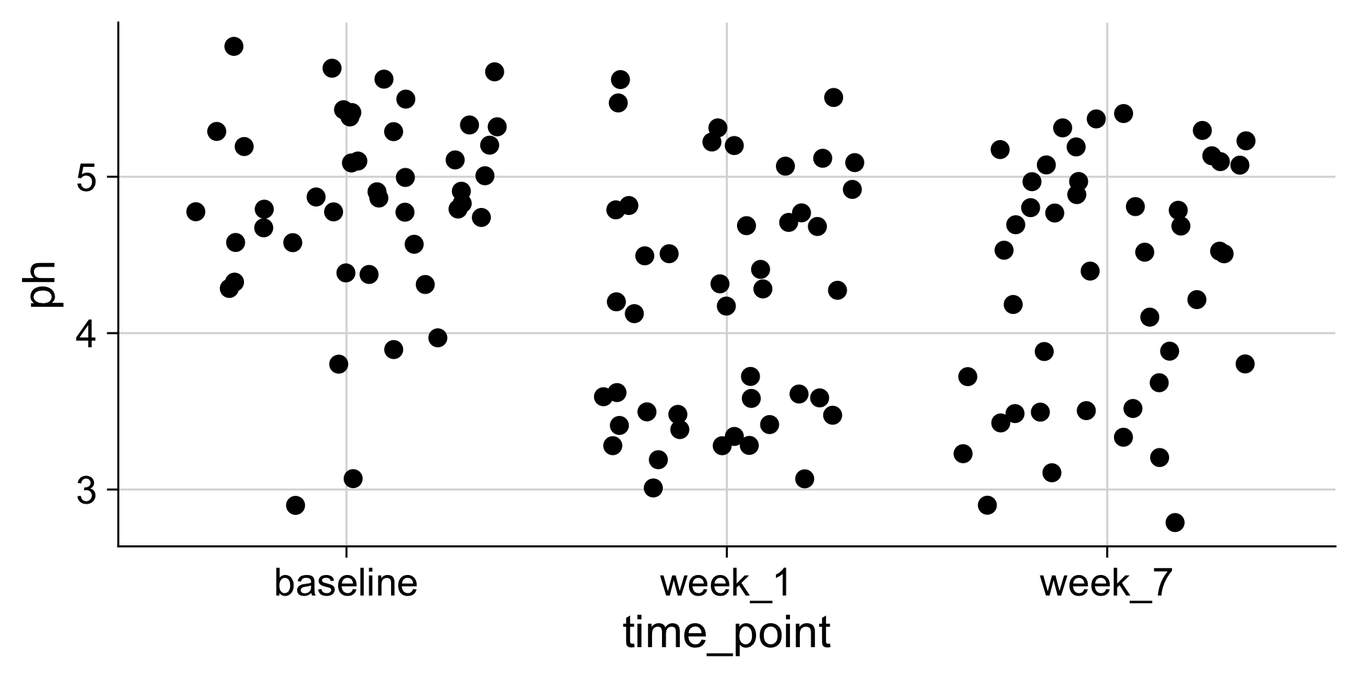
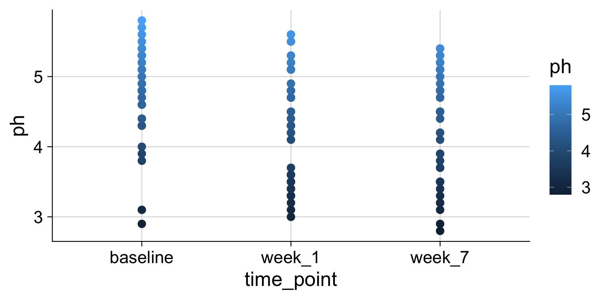
pH mapped to y position
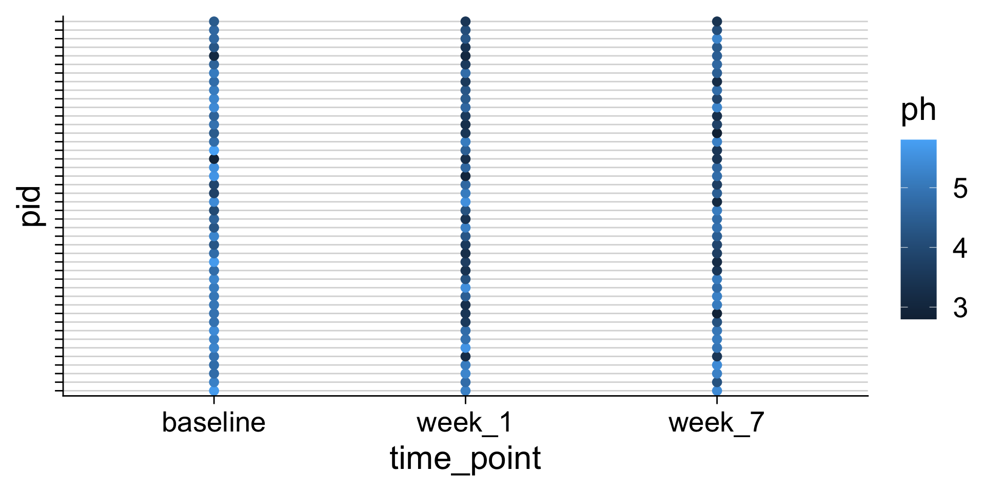
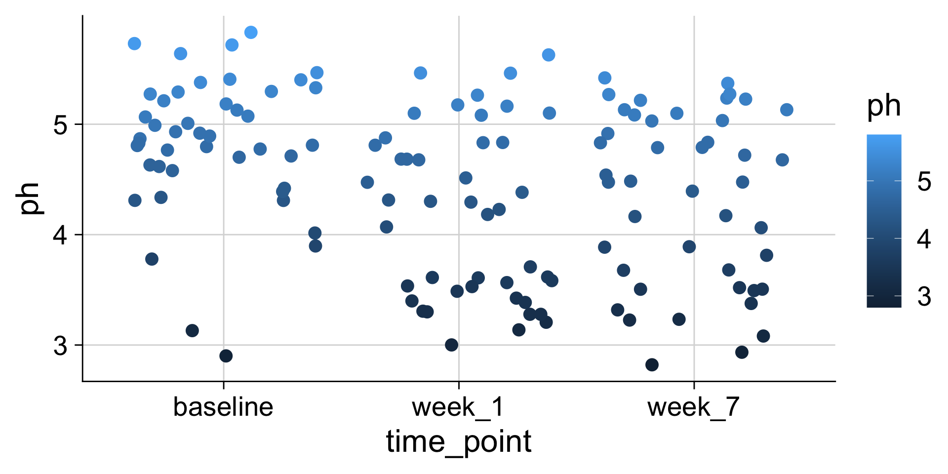
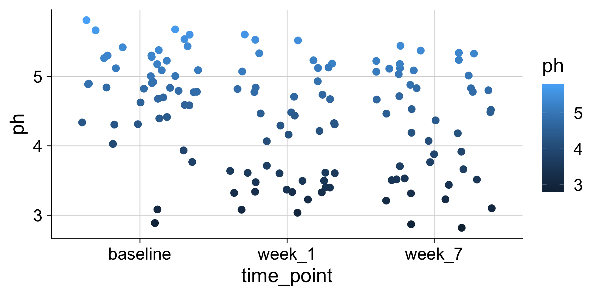
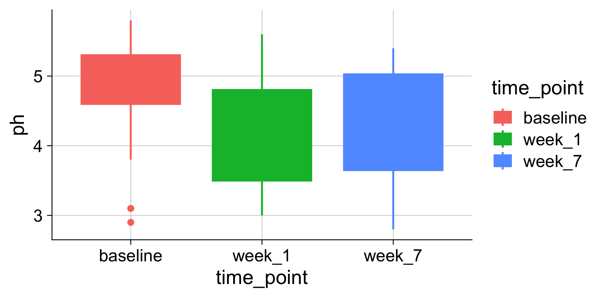
pH mapped to color
Commonly used aesthetics
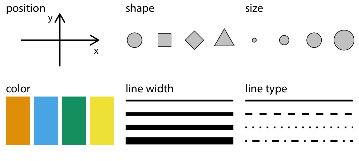
Figure from Claus O. Wilke. Fundamentals of Data Visualization. O’Reilly, 2019
The same data values can be mapped to different aesthetics
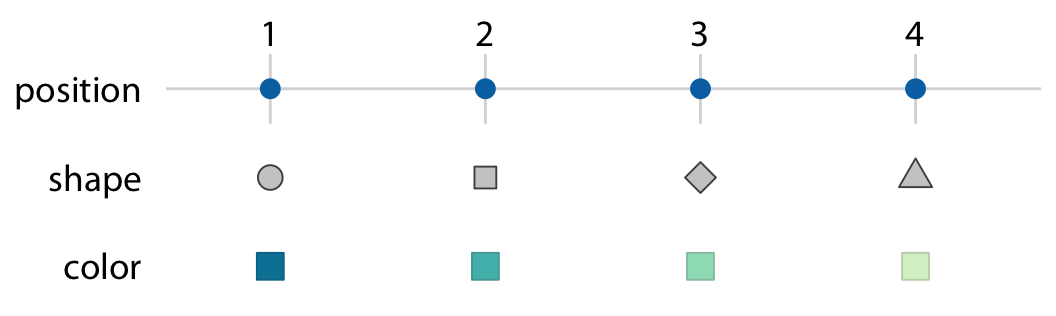
Figure from Claus O. Wilke. Fundamentals of Data Visualization. O’Reilly, 2019
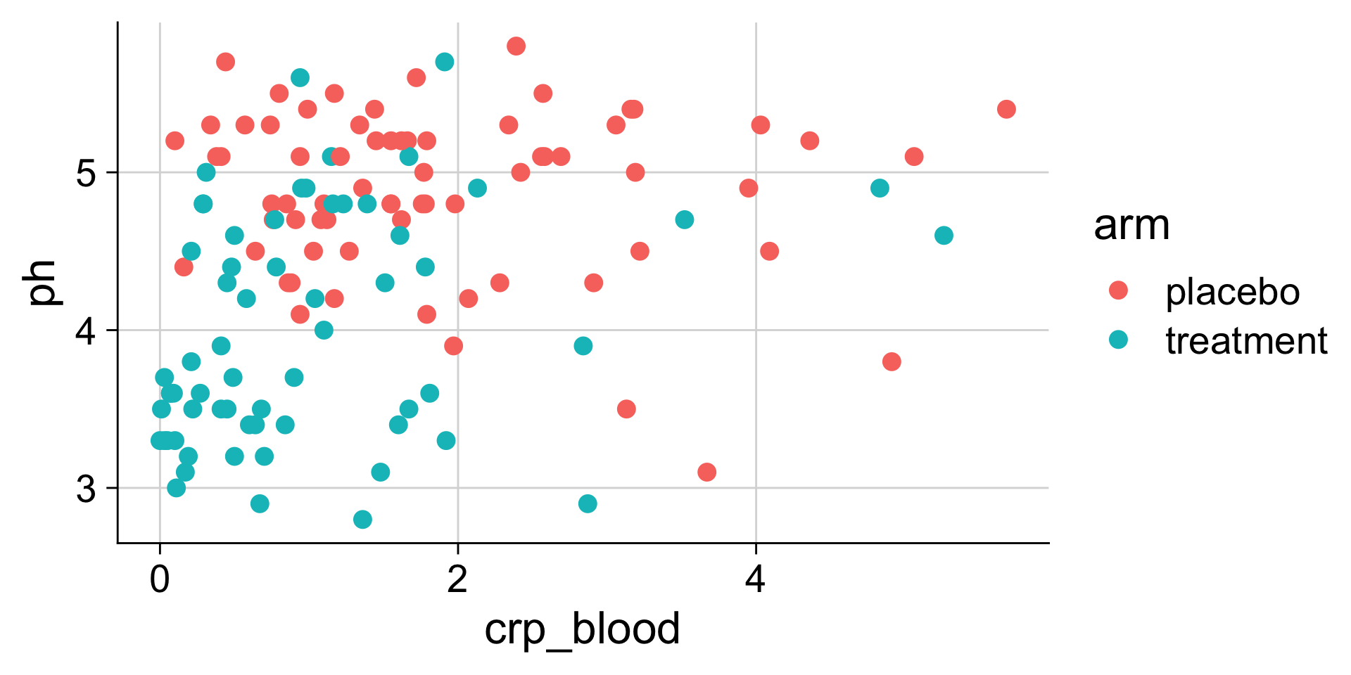
We can use many different aesthetics at once

We define the mapping with aes()
The geom determines how the data is shown
The geom determines how the data is shown
The geom determines how the data is shown
Different geoms have parameters for control
Different geoms have parameters for control
Many geoms have both color and fill aesthetics
Many geoms have both color and fill aesthetics
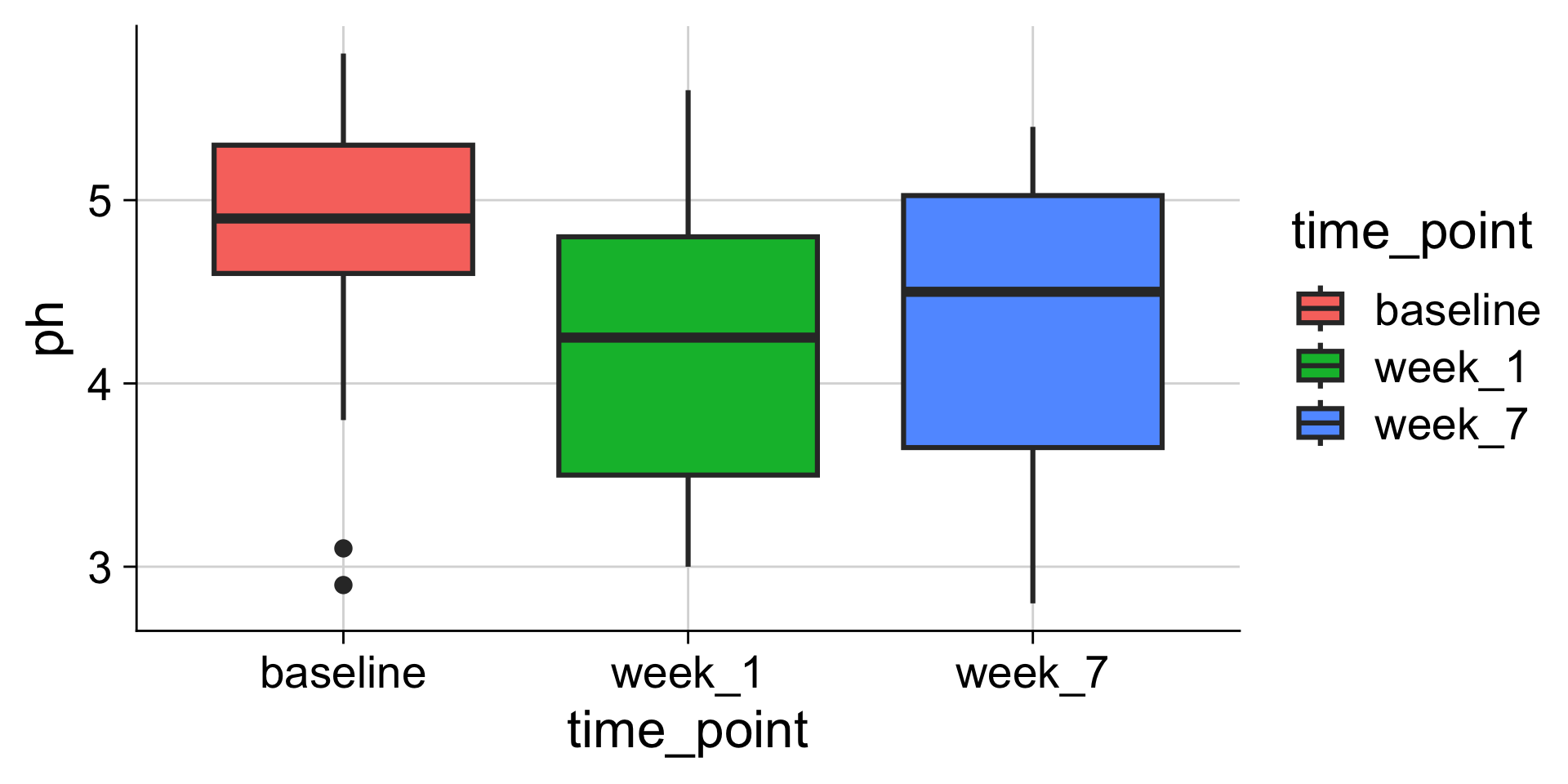
Many geoms have both color and fill aesthetics
Aesthetics can also be used as parameters in geoms

Aesthetics can also be used as parameters in geoms
Exercise
30:00
Time to try it yourself. Go to Exercise 3.
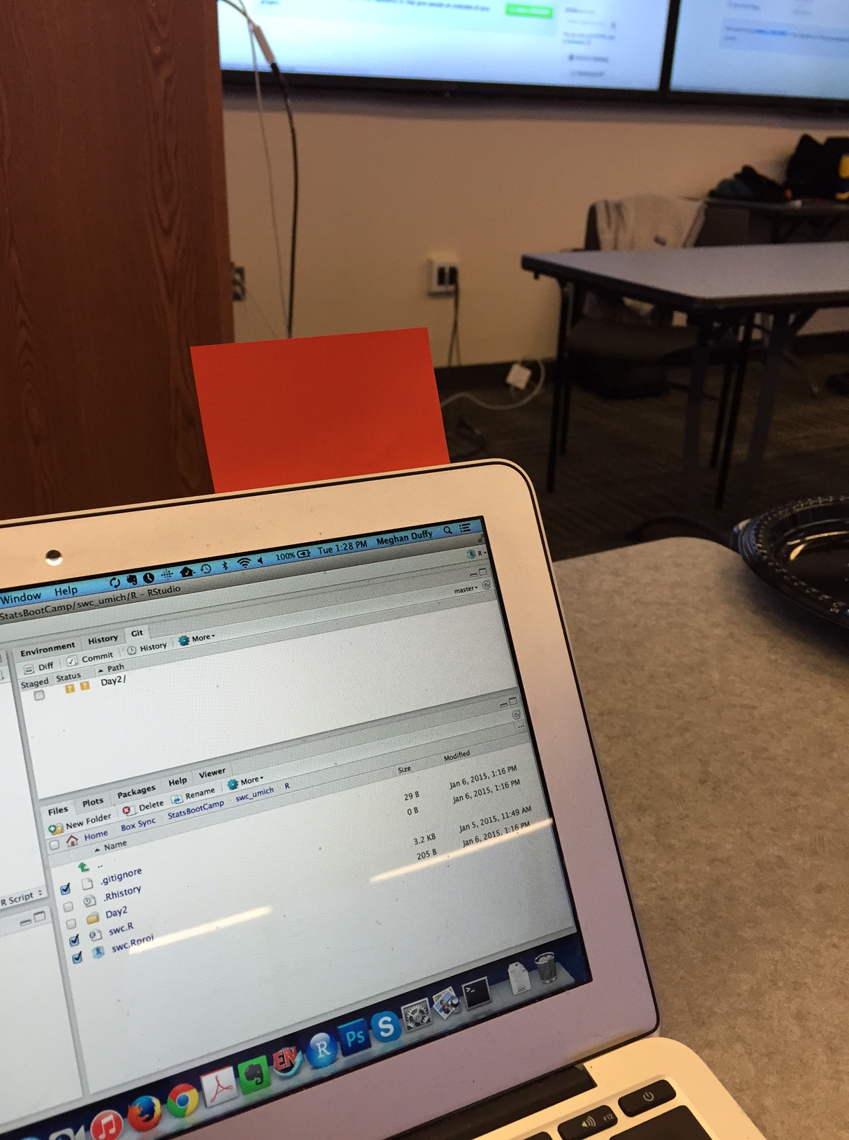
During an activity, place a yellow sticky on your laptop if you’re good to go and a pink sticky if you want help.
Histograms depend on the chosen bin width

Let’s take a poll
Go to the event on wooclap
Making histograms with ggplot: geom_histogram()
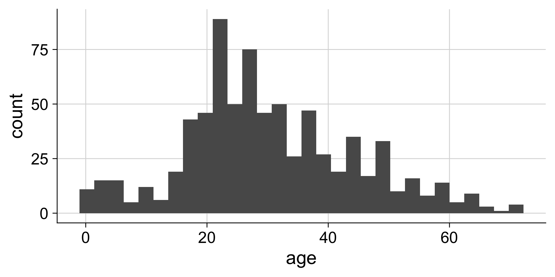
Setting the bin width
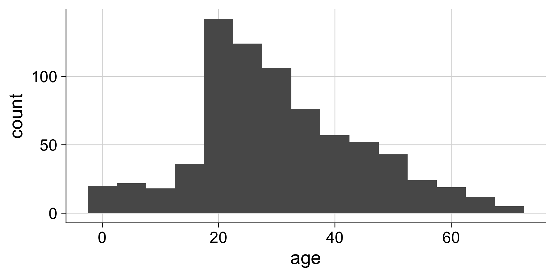
Do you like where there bins are? What does the first bin say?
Always set the center as well, to half the bin_width
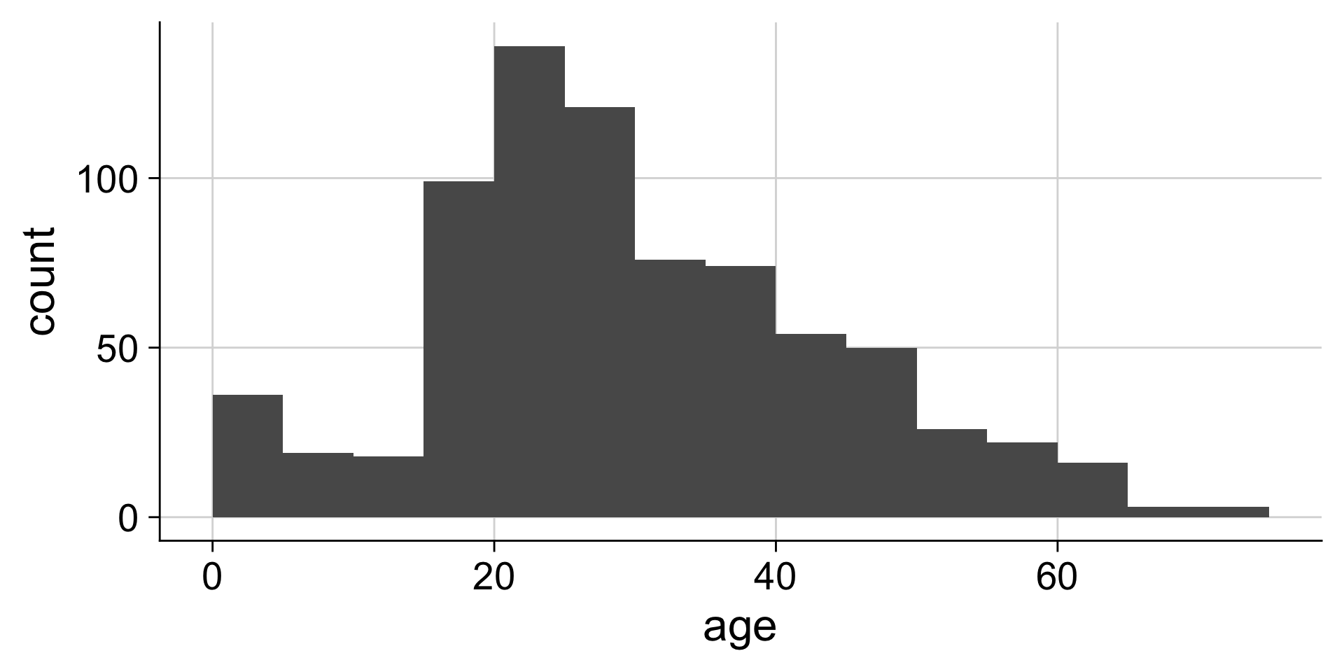
Setting center 2.5 makes the bars start 0-5, 5-10, etc. instead of 2.5-7.5, etc. You could instead use the argument boundary=5 to accomplish the same behavior.
Making density plots with ggplot: geom_density()
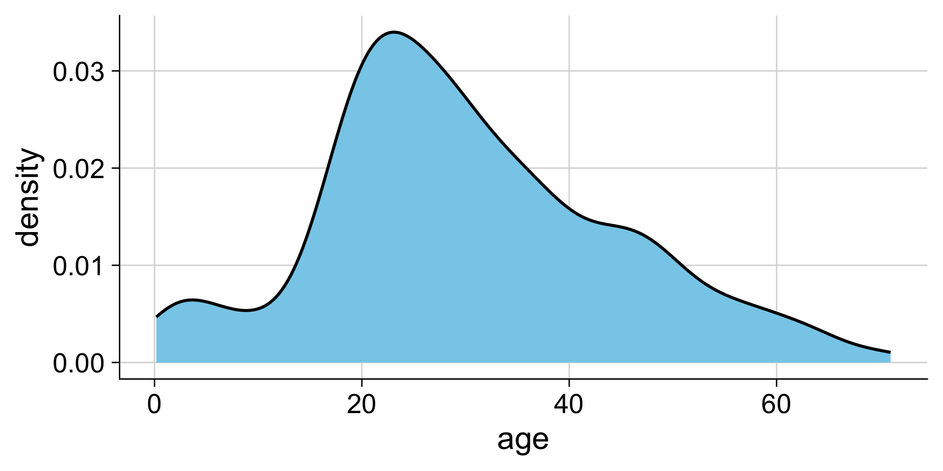
Making density plots with ggplot: geom_density()
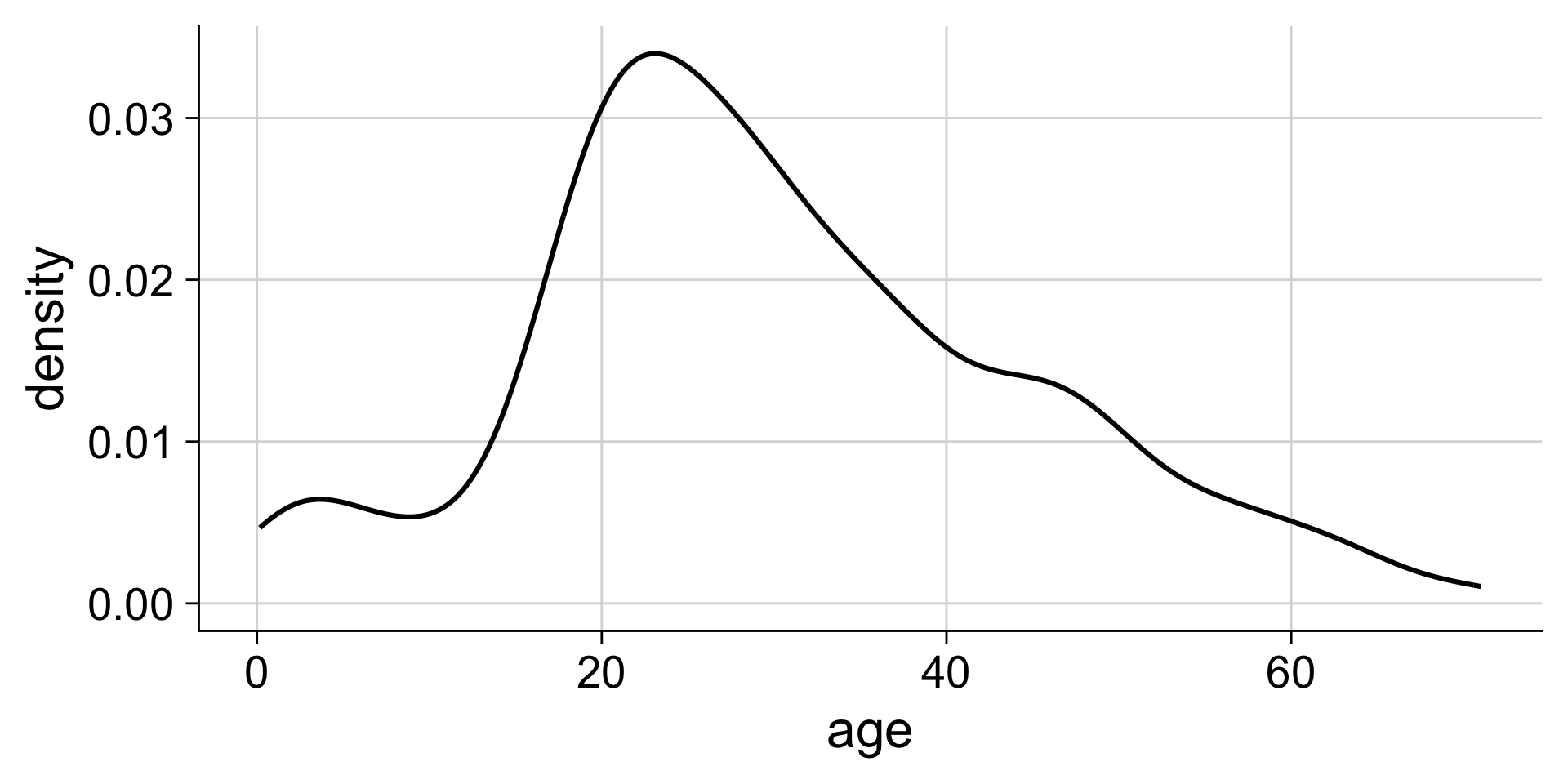
without fill
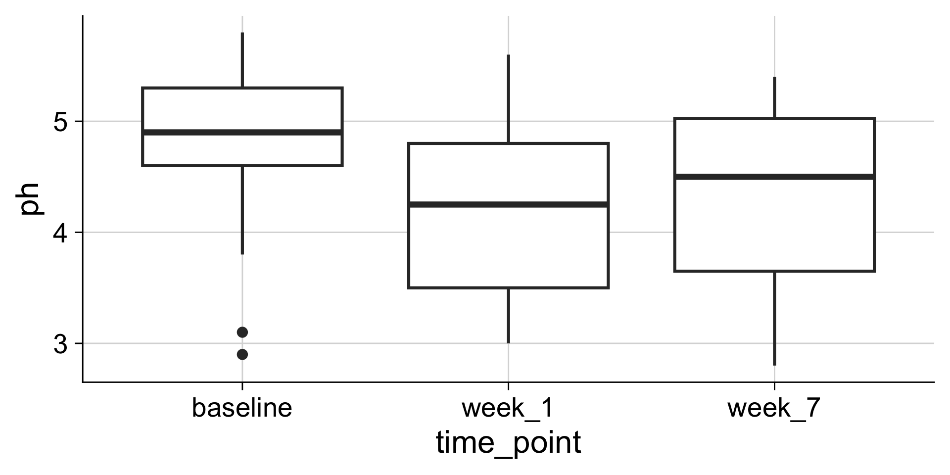
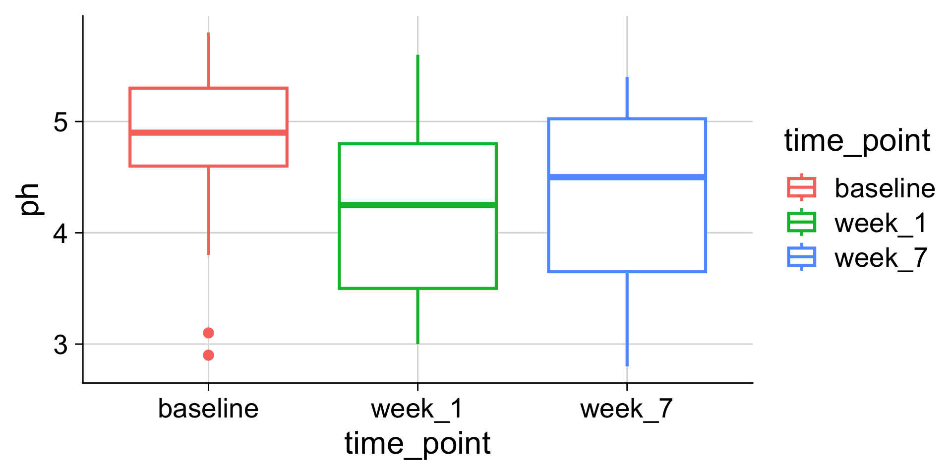
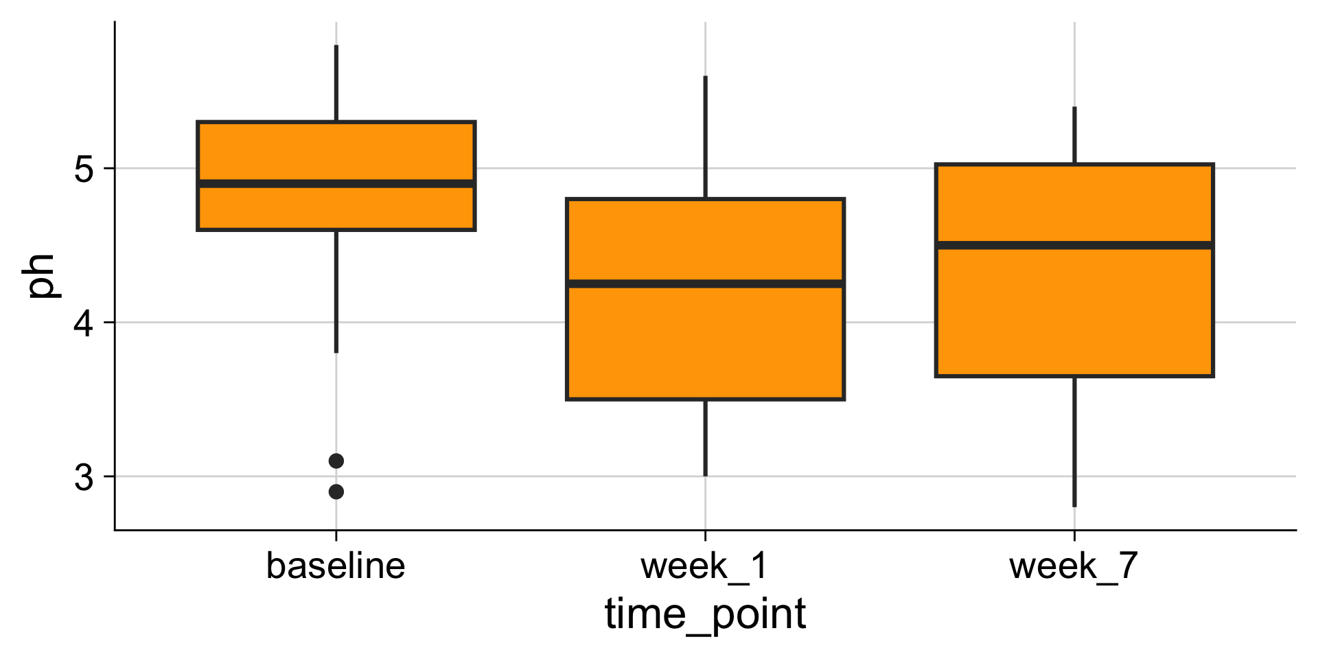
Boxplots: Showing values along y, conditions along x
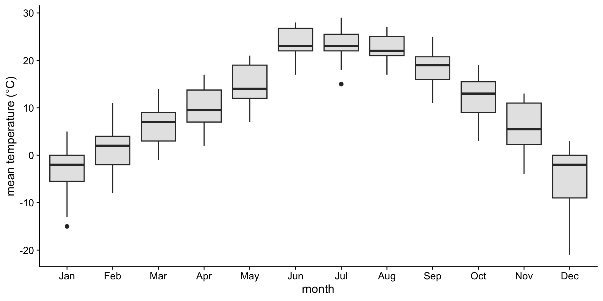
A boxplot is a crude way of visualizing a distribution.
How to read a boxplot

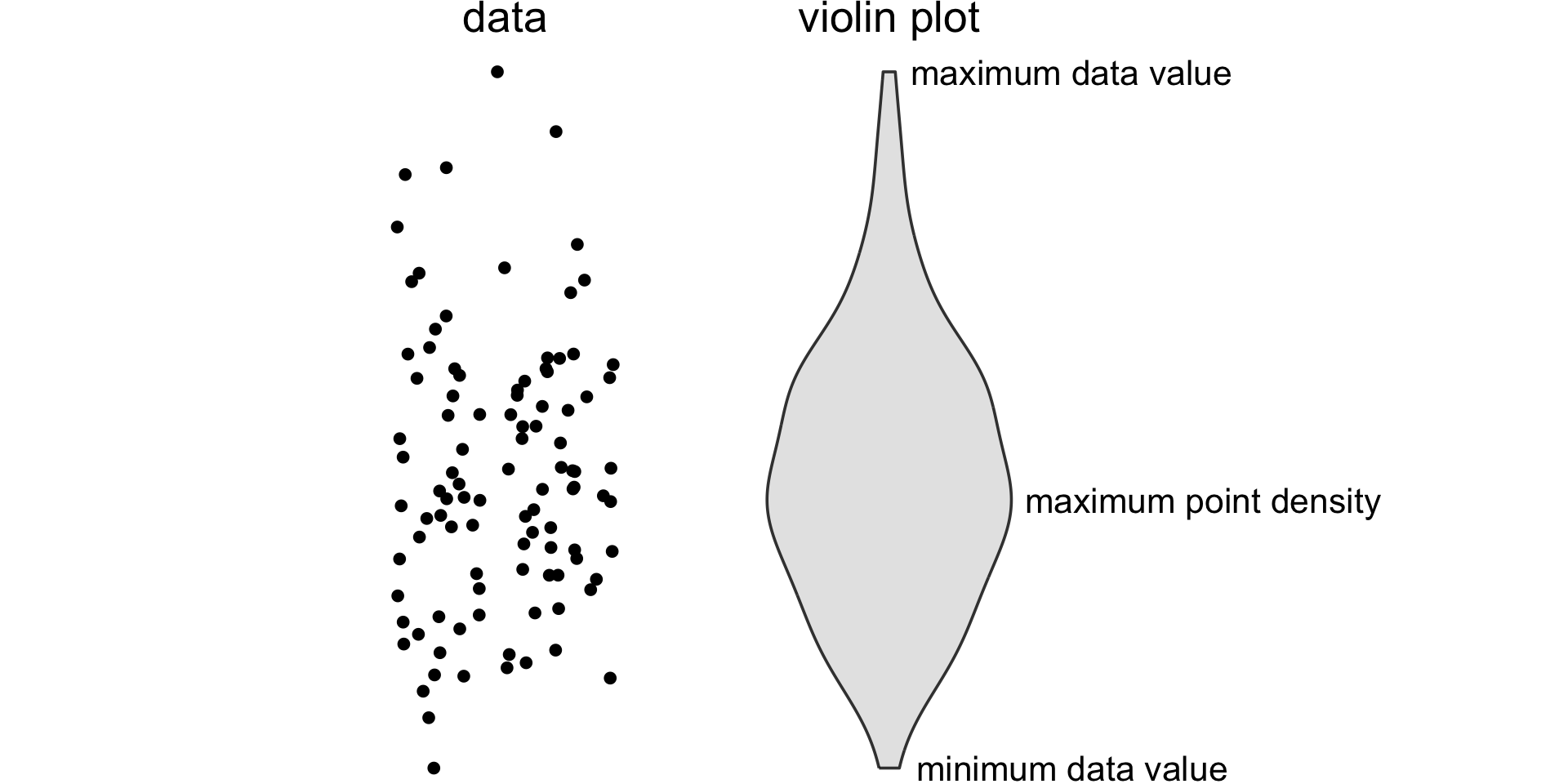
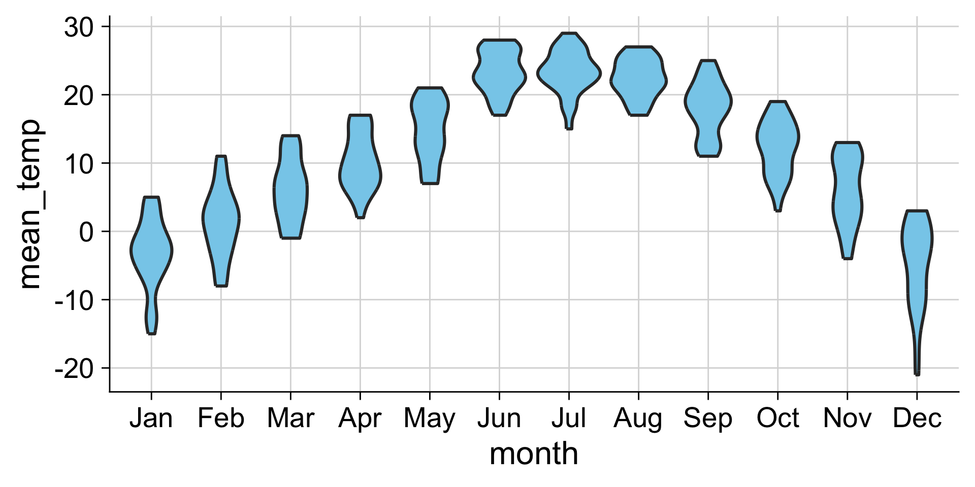
If you like density plots, consider violins
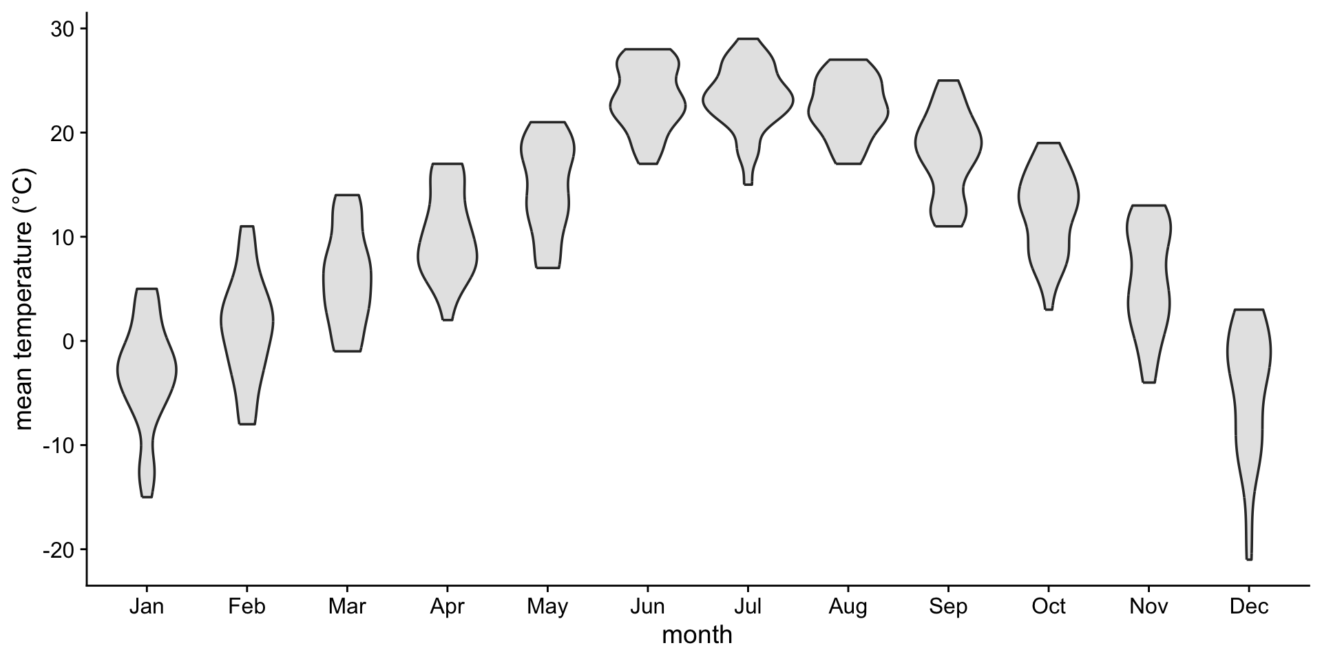
A violin plot is a density plot rotated 90 degrees and then mirrored.
How to read a violin plot
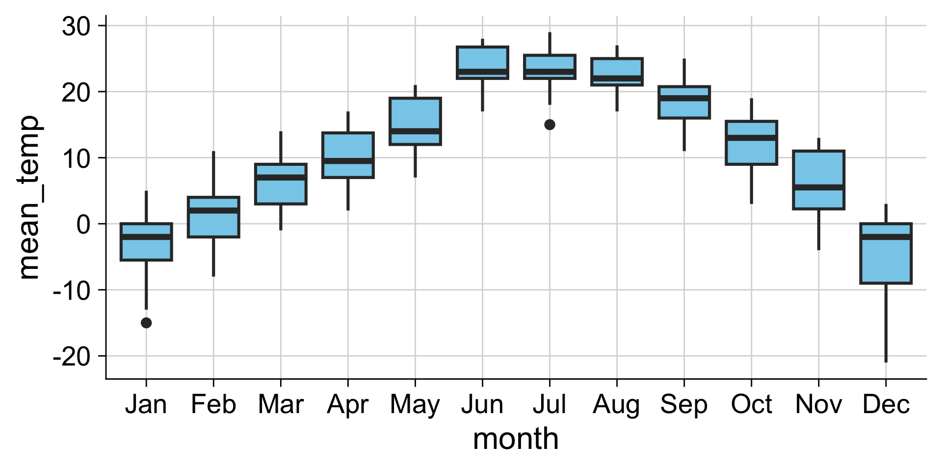
Examples: Boxplot
Examples: Violins
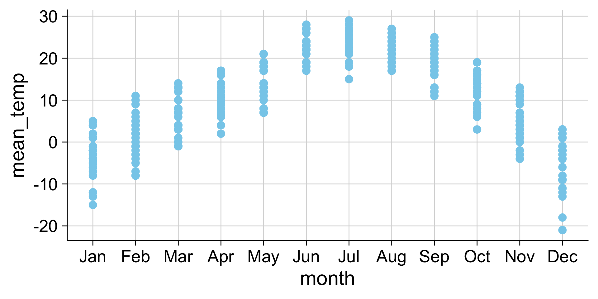
Examples: Strip chart (no jitter)
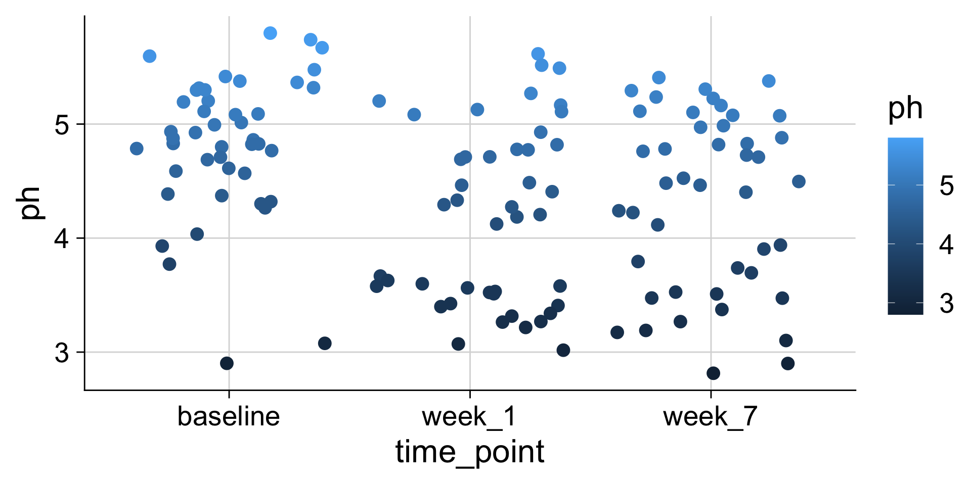
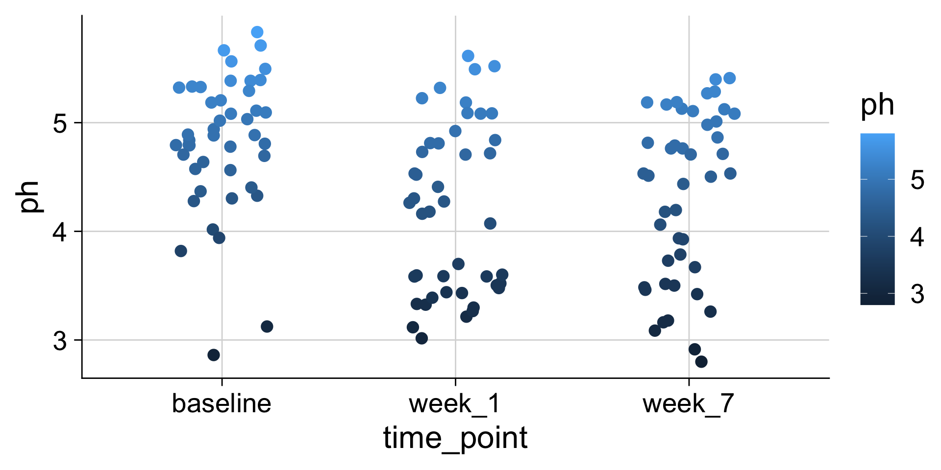
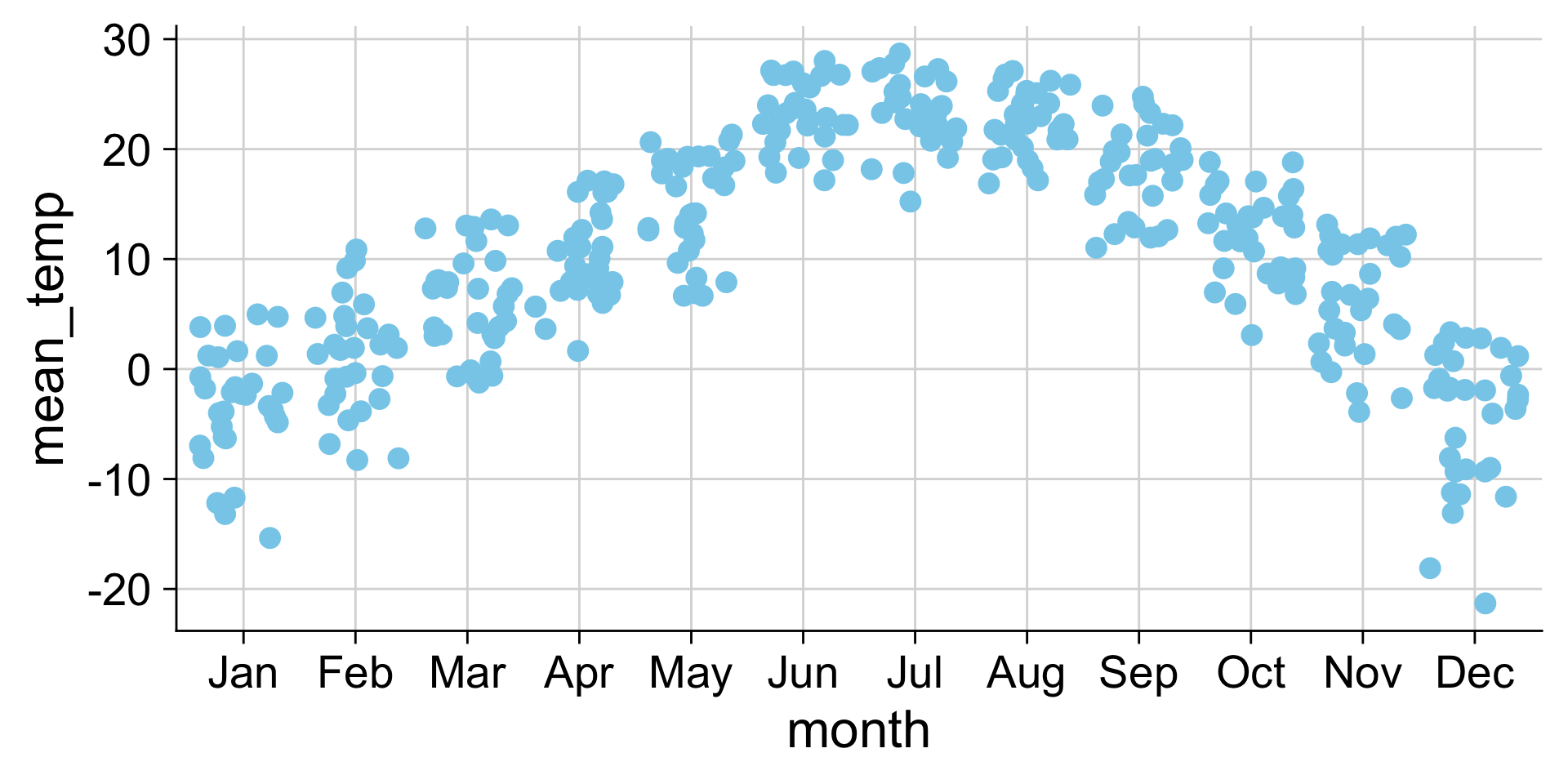
Examples: Strip chart (w/ jitter)
Analyze subsets: group_by() and summarize()

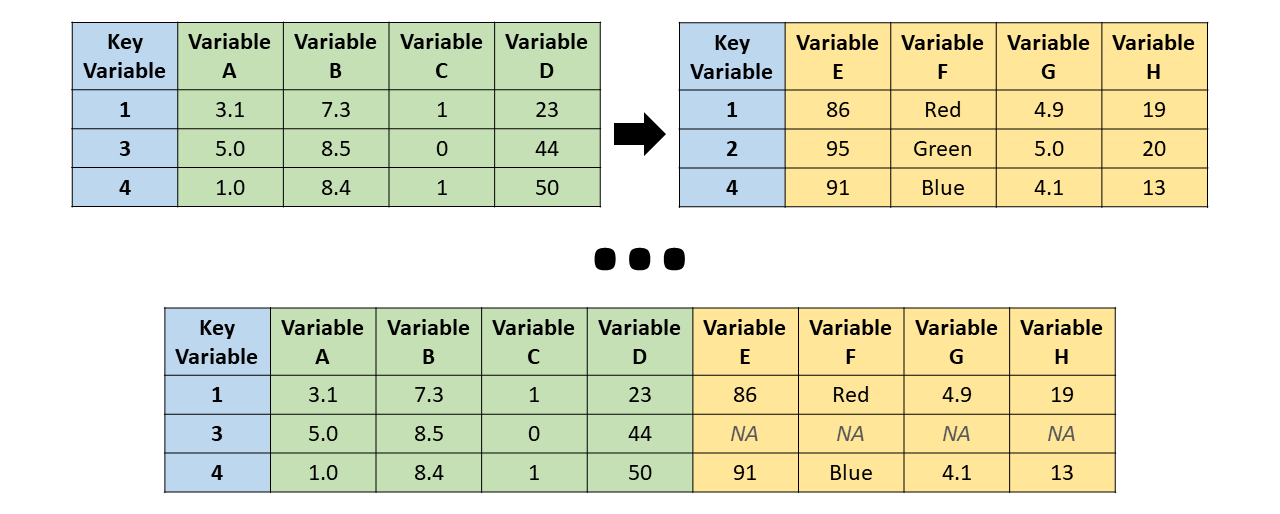
Reshape: pivot_wider() and pivot_longer()

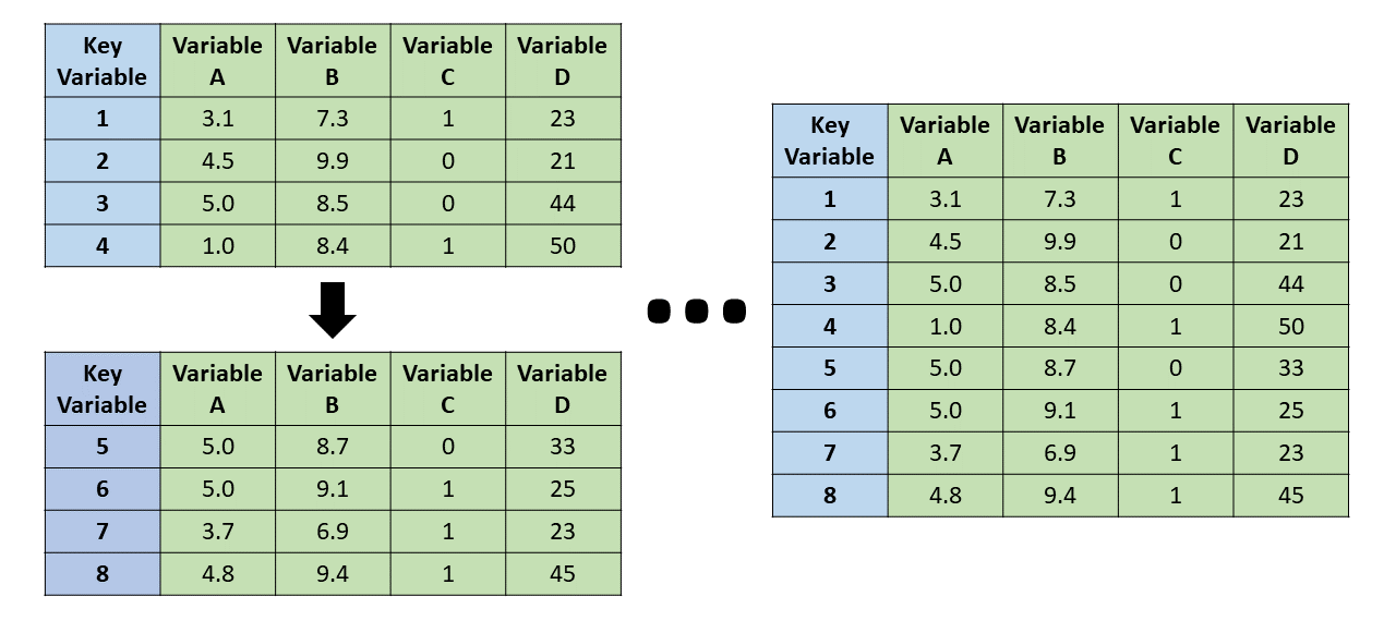
We use joins to add columns from one table into another

There are different types of joins
The differences are all about how to handle when the two tables have different key values

left_join() - the resulting table always has the same key_values as the “left” table
right_join() - the resulting table always has the same key_values as the “right” table
inner_join() - the resulting table always only keeps the key_values that are in both tables
full_join() - the resulting table always has all key_values found in both tables
Left Join
left_join() - the resulting table always has the same key_values as the “left” table
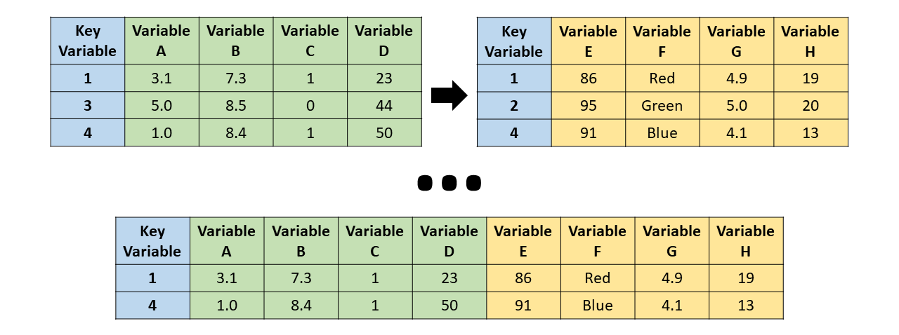
inner_join
inner_join() - the resulting table always only keeps the key_values that are in both tables
Note, merging tables vertically is bind_rows(), not a join