Background

Work in progress

Introduction to the pipeline

The goal of this pipeline is to take raw short-reads generated from an RNASeq library generation and sequencing protocol and do all the basic QC steps as well as quantify gene expression. Currently it only works for human RNAseq data - the reference data base is hard coded.

Inputs

This pipeline takes a sample sheet and fastq files (ideally in /n/groups/kwon/data1/sequencing_run_archive_DO_NOT_EDIT/) as input and works for both single and paired-end reads.

input `sample_sheet.csv` columns

sample	fastq_1	fastq_2	strandedness
Sample IDs	File path for forward reads	File path for reverse reads. If your sequences are single end, leave this column empty	Set as `auto` for each sample. However, for samples with high contaminants coming from smartseq2, it should be set as `both`.

See the walkthrough for information on how to make your samplesheet.

outputs: QC

After successfully running the pipeline, you will have a results folder in your project directory with the output from the pipeline.

First, take a look at the MultiQC report in /n/groups/kwon/johnathan/projects/simran_rnaseq/my_rnaseq_run/rnaseq_gene_expression-main/results/multiqc/star_salmon/nfcore_rnaseq_multiqc_report.html

You’ll see a summary table at the beginning:

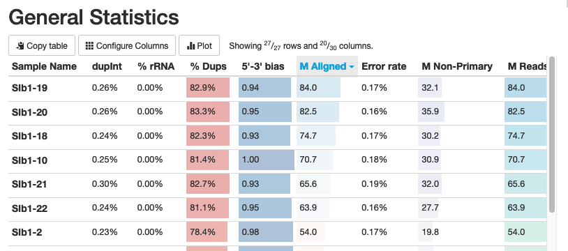
Here you want to check how many aligned sequences you had for each sample. You want 20-30 million reads per sample.

Also take a look at the breakdown of the types of sequences you got:

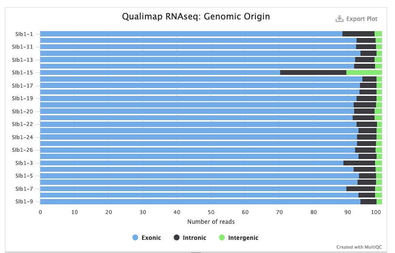
Depending on the type of library prep you did the might be different expectations here. But most library preps for gene expression analysis enrich for mature mRNA, so you should see mostly exonic reads.

For a comprehensive breakdown of the different QC plots you expect, check https://nf-co.re/rnaseq/dev/docs/output.

outputs: gene expression.

In the results/star_salmon folder, you’ll see a ton of folders and files. The main ones to focus on are:

star_salmon.merged.gene_counts.tsv: Matrix of gene-level raw counts across all samples.
star_salmon.gene_tpm.tsv: Matrix of gene-level TPM values across all samples.
star_salmon.merged.gene_lengths.tsv: Matrix of average within-sample transcript lengths for each gene across all samples.
star_salmon.merged.gene_counts_scaled.tsv: Matrix of gene-level library size-scaled estimated counts across all samples.

For import into DESeq2 we’ll use star_salmon.merged.gene_lengths.tsv . If you want to plot heatmaps and nromalized gene expression boxplots, use star_salmon.gene_tpm.tsv.

Beyond the pipeline

Typically you’ll want to explore your RNAseq dataset for more quality checks and sanity checks, and look for differences in gene expression with different treatments.

The following code is an example of how to get your data into deseq2. (Make sure you have the recommended packages installed by following the R installation instructions).

library(DESeq2)
library(tidyverse)
library(microViz)

counts <- read_tsv("salmon.merged.gene_counts_length_scaled.tsv")

counts_for_deseq <- counts %>% select(-gene_name) %>%
  as.data.frame() %>%
  column_to_rownames("gene_id") %>%
  as.matrix()

gene_names_for_deseq <- counts %>% select(gene_id, gene_name) %>%
  as.data.frame() %>%
  column_to_rownames("gene_id")

sample_metadata_for_deseq <- tibble(sample_id =  counts %>% select(-gene_id, -gene_name) %>% colnames()) %>% left_join (read_csv("SKH_Expt_P10_metadata.csv")) %>%
  as.data.frame() %>%
  column_to_rownames("sample_id")

deseq_dataset <- DESeqDataSetFromMatrix(countData=round(counts_for_deseq), colData=sample_metadata_for_deseq, rowData=gene_names_for_deseq, design=~treatment_code)

Then, read through and follow along with the DEseq2 vignette, starting with the “Pre-filtering” section.

As an example, here is a code chunk that combines the pre-filtering example and the PCA code from the vignette.

smallestGroupSize <- 3
keep <- rowSums(counts(deseq_dataset) >= 10) >= smallestGroupSize
dds <- deseq_dataset[keep,]

vsd <- vst(dds, blind=FALSE)
pcaData <- plotPCA(vsd, intgroup=c("polyamine", "inhibitor"), returnData=TRUE)
percentVar <- round(100 * attr(pcaData, "percentVar"))
ggplot(pcaData, aes(PC1, PC2, color=polyamine, shape=inhibitor)) +
  geom_point(size=3) +
  xlab(paste0("PC1: ",percentVar[1],"% variance")) +
  ylab(paste0("PC2: ",percentVar[2],"% variance")) + 
  coord_fixed()

`microViz` hack, largely untested.

This following code is a hack to get your already normalized data into a phyloseq object, which is typically only used for 16S analysis. However, there are very nice ordination functions and heatmap functions available for phyloseq objects in the microViz package, so it might be worth the hackiness.

library(microViz)
gene_abundance <- read_tsv("salmon.merged.gene_tpm.tsv")

gene_count_table <- gene_abundance %>%
  select(-gene_name) %>%
  as.data.frame() %>%
  column_to_rownames("gene_id") %>%
  as.matrix() %>%
  phyloseq::otu_table(taxa_are_rows = TRUE)

gene_annotations <- gene_abundance %>% select(gene_id, gene_name) %>%
  as.data.frame() %>%
  column_to_rownames("gene_id") %>%
  as.matrix() %>%
  phyloseq::tax_table()

sample_metadata <- tibble(sample_id =  counts %>% select(-gene_id, -gene_name) %>% colnames()) %>% left_join (read_csv("SKH_Expt_P10_metadata.csv")) %>%
  as.data.frame() %>%
  column_to_rownames("sample_id")
  phyloseq::sam_data()

rnaseq_dataset <- phyloseq::phyloseq(gene_count_table, gene_annotations, sample_metadata) %>% tax_fix()