library(tidyverse)
library(phyloseq)
library(microViz)
library(mixOmics)
library(factoextra)
library(corrplot)


metadata <- read_csv("../../datasets/multiomics_dataset/01_timepoint_metadata.csv")

cytokines <- read_csv("../../datasets/multiomics_dataset/03_cytokine_concentrations.csv")

microbiome <- read_csv("../../datasets/multiomics_dataset/02_16S_abundances.csv")Multi-omics primer
Resources
Workshop materials on 16S data processing and visualization Durban Data Science for Biology Workshop
microViz documentation available here
Modern Statistics for Modern Biology from Susan Holmes Wolfgang Huber
Slides: Multiomics primer
Slides: Full multiomics integration
Download the instructional dataset:
sample_id - sample id time_point - time point (week 18, week 24, week 34) pid - participant id
outcome - pregnancy outcome, either “term” or “preterm” amine_wt - Amsel criteria whiff test
disch - Amsel criteria discharge
clue_cells- Amsel criteria clue cells
p_h - Amsel criteria pH test
sample_id - sample id ... - each column is a bacterial taxa, with the contents being the counts of sequences in a sample assigned to that taxa
sample_id - sample id ... - each column is a cytokine, with the contents being the concentration of that cytokine in a sample
This is the taxonomic table in the right format to make a phyoloseq object from the 16S data.
Read this with readRDS('path/to/04_16s_taxa_table.RDS')
Beginnings of the live-coding session:
plotting one cytokine at a time - il_1a
cytokines %>%
    ggplot(aes(x=il_1a)) +
    geom_histogram() +
    scale_x_log10()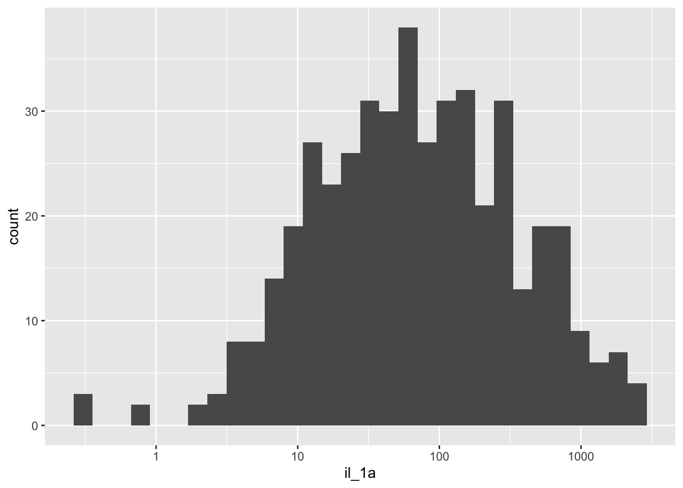
plotting all the cytokines
cytokines %>%
    pivot_longer(-sample_id, names_to="cytokine", values_to = "concentration") %>%
    ggplot(aes(x=concentration)) +
    geom_histogram() +
    scale_x_log10() +
    facet_wrap(~cytokine, scales="free")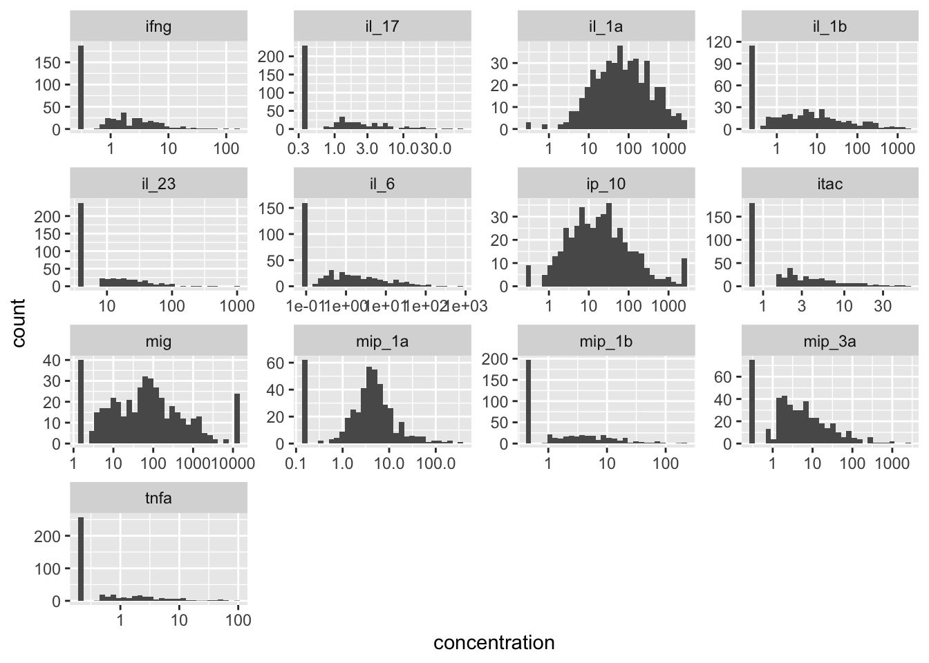
Are my cytokines correlated?
Plotting one pair at a time
cytokines %>%
    ggplot(aes(x=il_1a, y=ip_10)) +
    geom_point() +
    scale_y_log10() +
    scale_x_log10() +
    geom_smooth(method="lm", se=TRUE)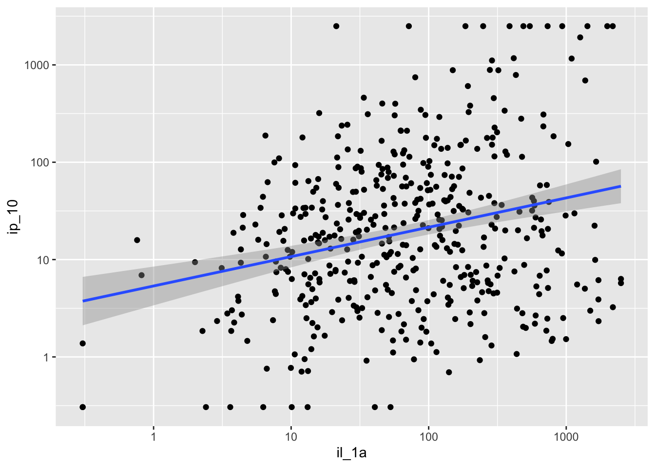
plot all the correlations using corplot
cytokine_cor_matrix <- cytokines %>%
    as.data.frame() %>%
    column_to_rownames("sample_id") %>%
    as.matrix() %>%
    cor(method="spearman")

corrplot(cytokine_cor_matrix,
         method = "color",
         type = "upper",           # Show only upper triangle
         order = "hclust",         # Cluster similar peptides
         addCoef.col = "black",    # Add correlation coefficients
         tl.col = "black",         # Text label color
         tl.srt = 45,              # Rotate text labels 45 degrees
         diag = FALSE)             # Hide diagonal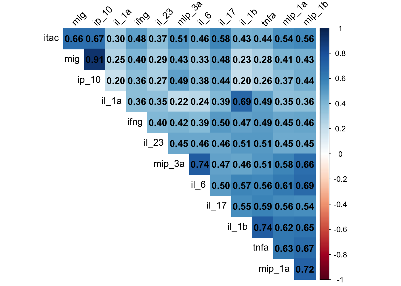
should we do dimensionality reduction?
pca_result <- cytokines %>%
    as.data.frame() %>%
    column_to_rownames("sample_id") %>%
    as.matrix() %>%
    log10() %>%
    prcomp(scale. = TRUE, center = TRUE)


# Scree plot
fviz_eig(pca_result, addlabels = TRUE)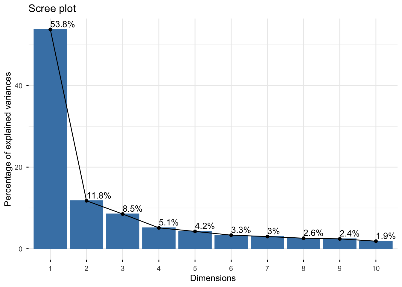
# Biplot with better aesthetics
fviz_pca_biplot(pca_result,
                repel = TRUE,           # Avoid text overlap
                geom = c("point"),
                col.var = "red",        # Variables color
                col.ind = "blue",       # Individuals color
                title = "PCA Biplot - Cytokine Concentrations")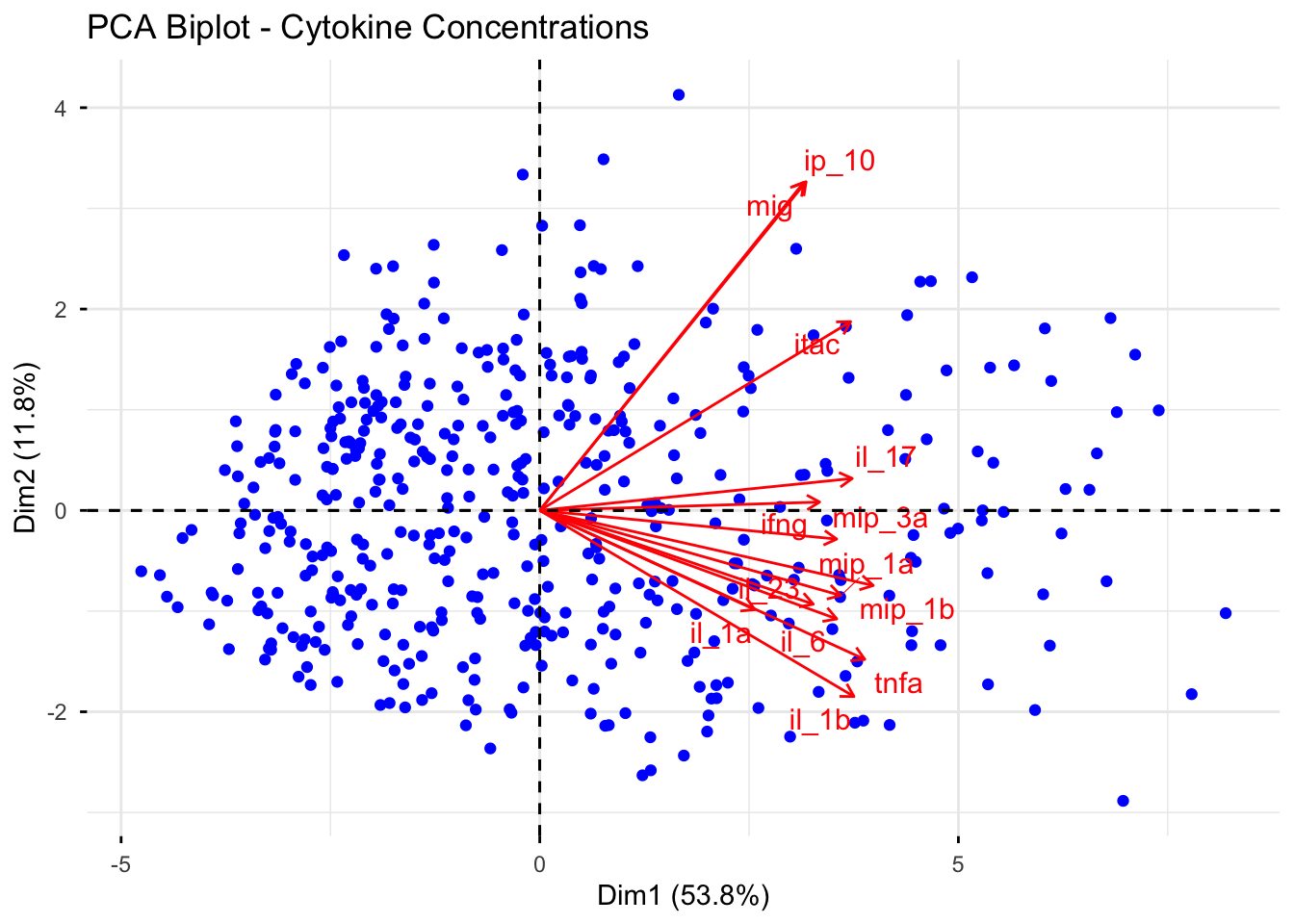
ps_count_table <- microbiome %>%
column_to_rownames("sample_id") %>%
as.matrix() %>%
phyloseq::otu_table(taxa_are_rows = FALSE)
ps_sample_data <- metadata %>%
left_join(cytokines) %>% #integration!
column_to_rownames("sample_id") %>%
phyloseq::sample_data()
ps_taxa_table <- readRDS("../../datasets/multiomics_dataset/04_16s_taxa_table.RDS")
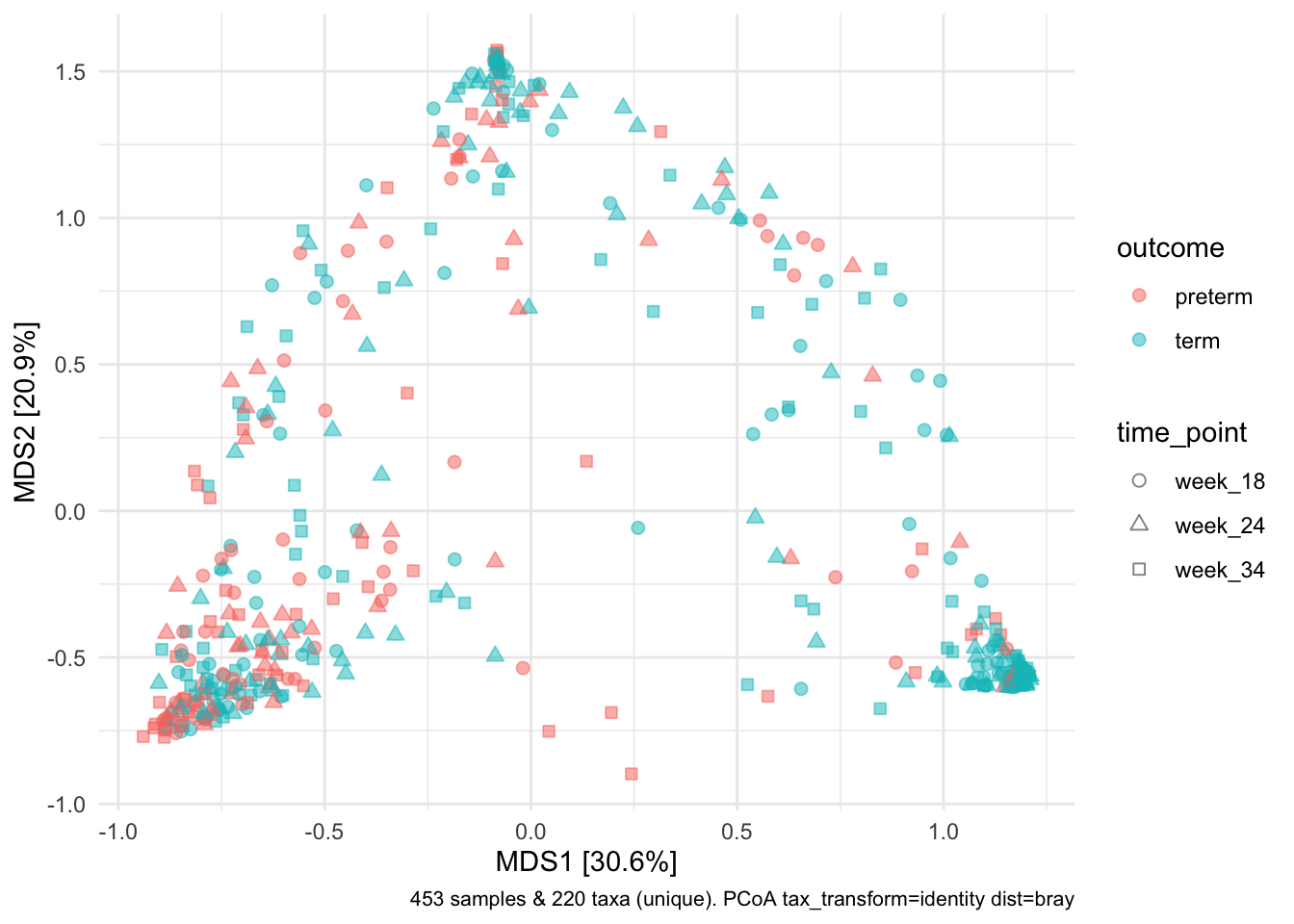
my_ps <- phyloseq(ps_count_table,ps_sample_data,ps_taxa_table)Let’s use Bray-Curtis distance, which is less sensitive to rare taxa changing and weights more abundant taxa higher than something like Euclidean distance.
my_ps %>%
 tax_transform(rank = "unique", trans = "identity") %>%
 dist_calc(dist = "bray") %>%
 ord_calc(
  method = "auto"
 ) %>%
 ord_plot(
  axes = c(1, 2),
  colour = "outcome", fill = "outcome",
  shape = "time_point", alpha = 0.5,
  size = 2
 ) +
 scale_shape_girafe_filled()